简介
在本教程中,我们将通过利用最适合每个时间序列的模型来探索在M5数据集上进行预测的过程。我们将通过一种称为交叉验证的基本技术来实现这一目标。这种方法有助于我们估计模型的预测性能,并选择为每个时间序列提供最佳性能的模型。
M5数据集包含了沃尔玛五年的分层销售数据。目标是预测未来28天的日销售额。该数据集按照美国的50个州进行了细分,每个州有10家商店。
在时间序列预测和分析领域中,较为复杂的任务之一是确定最适合特定系列的模型。很多时候,这个选择过程很大程度上依赖直觉,但这可能并不一定与我们数据集的实证现实相一致。
在本教程中,我们旨在为M5基准数据集中不同系列的模型选择提供更加结构化、数据驱动的方法。这个数据集在预测领域中非常著名,它能够展示我们方法的多样性和强大性。
我们将从各种预测范式中训练一系列模型:
(1) StatsForecast
- 基准模型:这些模型简单但通常非常有效,可以为预测问题提供初始视角。我们将在此类别中使用 SeasonalNaive 和 HistoricAverage 模型。
- 间歇模型:对于具有零散、不连续需求的序列,我们将使用 CrostonOptimized 、 IMAPA 和 ADIDA 等模型。这些模型特别适用于处理零膨胀序列。
- 状态空间模型:这些是使用系统的数学描述进行预测的统计模型。statsforecast库中的 AutoETS 模型属于这个类别。
(2) MLForecast
机器学习:利用 LightGBM 、 XGBoost 和 LinearRegression 等ML模型可以有优势,因为它们能够揭示数据中的复杂模式。我们将使用MLForecast库来实现这个目的。
(3) NeuralForecast
深度学习:DL模型,如Transformers( AutoTFT )和神经网络( AutoNHITS ),使我们能够处理时间序列数据中的复杂非线性依赖关系。我们将利用NeuralForecast库来使用这些模型。
使用Nixtla套件库,我们将能够通过数据驱动我们的模型选择过程,确保我们在数据集中针对特定系列使用最合适的模型。
大纲:
- 读取数据:在这个初始步骤中,我们将数据集加载到内存中,以便后续的分析和预测。在这个阶段,了解数据集的结构和细微差别非常重要。
- 使用统计和深度学习方法进行预测:我们应用了从基本统计技术到先进的深度学习模型的广泛预测方法。目标是基于我们的数据集生成未来28天的预测。
- 不同窗口上的模型性能评估:我们评估我们的模型在不同窗口上的性能。
- 选择一组序列的最佳模型:使用性能评估,我们为每组序列确定最优模型。这一步骤确保所选择的模型适应每个组的独特特征。
- 筛选最佳预测结果:最后,我们通过筛选我们选择的模型生成的预测结果,得到最有希望的预测。这是我们的最终输出,代表了根据我们的模型得出的每个系列的最佳可能预测。
此教程最初是在一个 c5d.24xlarge EC2 实例上执行的。
准备工作
安装库
!pip install statsforecast mlforecast neuralforecast datasetforecast s3fs pyarrow
下载并准备数据
该示例使用M5数据集。它由 30,490 个底部时间序列组成。
import pandas as pd
# Load the training target dataset from the provided URL
Y_df = pd.read_parquet('https://m5-benchmarks.s3.amazonaws.com/data/train/target.parquet')

# Rename columns to match the Nixtlaverse's expectations
# The 'item_id' becomes 'unique_id' representing the unique identifier of the time series
# The 'timestamp' becomes 'ds' representing the time stamp of the data points
# The 'demand' becomes 'y' representing the target variable we want to forecast
Y_df = Y_df.rename(columns={
    'item_id': 'unique_id',
    'timestamp': 'ds',
    'demand': 'y'
})

# Convert the 'ds' column to datetime format to ensure proper handling of date-related operations in subsequent steps
Y_df['ds'] = pd.to_datetime(Y_df['ds'])
为简单起见,我们将只保留一个类别
Y_df = Y_df.query('unique_id.str.startswith("FOODS_3")').reset_index(drop=True)

Y_df['unique_id'] = Y_df['unique_id'].astype(str)
基本绘图
使用 StatsForecast 类的plot方法绘制一些系列。该方法从数据集中打印出8个随机序列,对基本的探索性数据分析很有用。
from statsforecast import StatsForecast
# Feature: plot random series for EDA
StatsForecast.plot(Y_df)
# Feature: plot groups of series for EDA
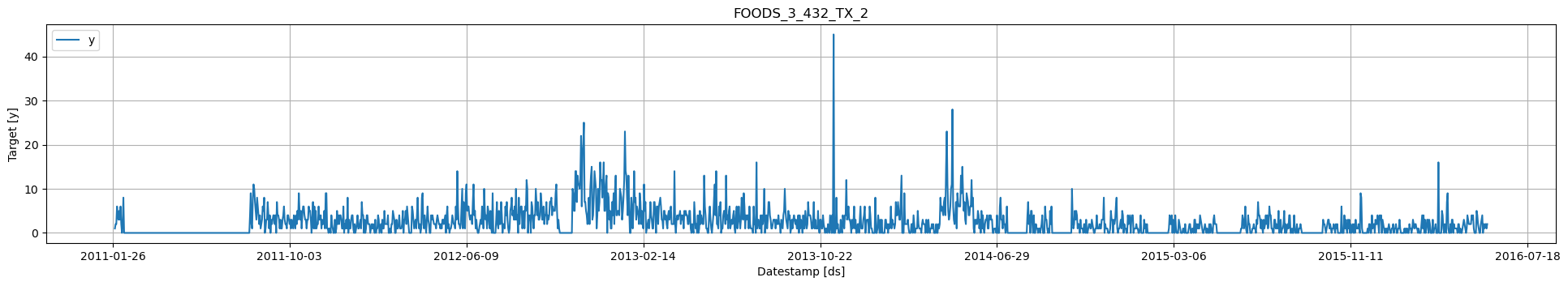
StatsForecast.plot(Y_df, unique_ids=["FOODS_3_432_TX_2"])
# Feature: plot groups of series for EDA
StatsForecast.plot(Y_df, unique_ids=["FOODS_3_432_TX_2"], engine ='matplotlib')
使用统计、机器学习和神经方法创建预测
StatsForecast
StatsForecast 是一个综合性的库,提供了一套流行的单变量时间序列预测模型,所有模型都专注于高性能和可扩展性。
以下是使StatsForecast成为时间序列预测强大工具的原因:
- 本地模型集合:StatsForecast提供了多样化的本地模型,可以分别应用于每个时间序列,使我们能够捕捉到每个序列中的独特模式。
- 简洁性:使用StatsForecast,训练、预测和回测多个模型变得简单直接,只需要几行代码。这种简洁性使其成为初学者和经验丰富的从业者的便利工具。
- 针对速度进行优化:StatsForecast中的模型实现经过速度优化,确保大规模计算高效执行,从而减少模型训练和预测的总时间。
- 水平可扩展性:StatsForecast的一个显著特点是其水平扩展能力。它与Spark、Dask和Ray等分布式计算框架兼容。该特性使其能够通过在集群中的多个节点上分布计算来处理大型数据集,使其成为大规模时间序列预测任务的首选解决方案。
StatsForecast 每次接收到要拟合的模型列表。由于我们处理的是每日数据,使用7作为季节性将是有益的。
# Import necessary models from the statsforecast library
from statsforecast.models import (
    # SeasonalNaive: A model that uses the previous season's data as the forecast
    SeasonalNaive,
    # Naive: A simple model that uses the last observed value as the forecast
    Naive,
    # HistoricAverage: This model uses the average of all historical data as the forecast
    HistoricAverage,
    # CrostonOptimized: A model specifically designed for intermittent demand forecasting
    CrostonOptimized,
    # ADIDA: Adaptive combination of Intermittent Demand Approaches, a model designed for intermittent demand
    ADIDA,
    # IMAPA: Intermittent Multiplicative AutoRegressive Average, a model for intermittent series that incorporates autocorrelation
    IMAPA,
    # AutoETS: Automated Exponential Smoothing model that automatically selects the best Exponential Smoothing model based on AIC
    AutoETS
)
我们通过使用以下参数实例化一个新的StatsForecast对象来拟合模型:
- models :模型列表。从模型中选择您想要的模型并导入。
- freq :一个表示数据频率的字符串。(请参阅pandas提供的可用频率)
- n_jobs :int,用于并行处理的作业数量,使用-1表示使用所有核心。
- fallback_model :如果模型失败,将使用该模型。任何设置都传递给构造函数。然后调用其fit方法并传入历史数据框。
horizon = 28
models = [
    SeasonalNaive(season_length=7),
    Naive(),
    HistoricAverage(),
    CrostonOptimized(),
    ADIDA(),
    IMAPA(),
    AutoETS(season_length=7)
]
# Instantiate the StatsForecast class
sf = StatsForecast(
    models=models,  # A list of models to be used for forecasting
    freq='D',  # The frequency of the time series data (in this case, 'D' stands for daily frequency)
    n_jobs=-1,  # The number of CPU cores to use for parallel execution (-1 means use all available cores)
)
预测方法接受两个参数:预测下一个h(时间段)和水平。
- h (int):表示未来预测的h步。在这种情况下,是提前12个月。
- level (浮点数列表):此可选参数用于概率预测。设置预测区间的水平(或置信度百分位)。例如,level=[90] 表示模型预计真实值在该区间内的概率为90%。
这里的预测对象是一个新的 data frame,其中包括一个带有模型名称和y hat值的列,以及用于表示不确定性区间的列。
这段代码计算运行StatsForecast类的预测函数所需的时间,该函数预测未来的28天(h=28)。级别设置为[90],表示将计算90%的预测区间。时间以分钟计算,并在最后打印出来。
from time import time

# Get the current time before forecasting starts, this will be used to measure the execution time
init = time()

# Call the forecast method of the StatsForecast instance to predict the next 28 days (h=28)
# Level is set to [90], which means that it will compute the 90% prediction interval
fcst_df = sf.forecast(df=Y_df, h=28, level=[90])

# Get the current time after the forecasting ends
end = time()

# Calculate and print the total time taken for the forecasting in minutes
print(f'Forecast Minutes: {(end - init) / 60}')
fcst_df.head()
| unique_id | ds | SeasonalNaive | SeasonalNaive-lo-90 | SeasonalNaive-hi-90 | Naive | Naive-lo-90 | Naive-hi-90 | HistoricAverage | HistoricAverage-lo-90 | HistoricAverage-hi-90 | CrostonOptimized | ADIDA | IMAPA | AutoETS | AutoETS-lo-90 | AutoETS-hi-90 |
|---|---|---|---|---|---|---|---|---|---|---|---|---|---|---|---|---|
| FOODS_3_001_CA_1 | 2016-05-23 | 1.0 | -2.847174 | 4.847174 | 2.0 | 0.098363 | 3.901637 | 0.448738 | -1.009579 | 1.907055 | 0.345192 | 0.345477 | 0.347249 | 0.381414 | -1.028122 | 1.790950 |
| FOODS_3_001_CA_1 | 2016-05-24 | 0.0 | -3.847174 | 3.847174 | 2.0 | -0.689321 | 4.689321 | 0.448738 | -1.009579 | 1.907055 | 0.345192 | 0.345477 | 0.347249 | 0.286933 | -1.124136 | 1.698003 |
| FOODS_3_001_CA_1 | 2016-05-25 | 0.0 | -3.847174 | 3.847174 | 2.0 | -1.293732 | 5.293732 | 0.448738 | -1.009579 | 1.907055 | 0.345192 | 0.345477 | 0.347249 | 0.334987 | -1.077614 | 1.747588 |
| FOODS_3_001_CA_1 | 2016-05-26 | 1.0 | -2.847174 | 4.847174 | 2.0 | -1.803274 | 5.803274 | 0.448738 | -1.009579 | 1.907055 | 0.345192 | 0.345477 | 0.347249 | 0.186851 | -1.227280 | 1.600982 |
| FOODS_3_001_CA_1 | 2016-05-27 | 0.0 | -3.847174 | 3.847174 | 2.0 | -2.252190 | 6.252190 | 0.448738 | -1.009579 | 1.907055 | 0.345192 | 0.345477 | 0.347249 | 0.308112 | -1.107548 | 1.723771 |
MLForecast
MLForecast 是一个强大的库,为时间序列预测提供自动化特征创建功能,便于使用全局机器学习模型。它专为高性能和可扩展性而设计。
MLForecast的主要特点包括:
- 支持sklearn模型:MLForecast与遵循scikit-learn API的模型兼容。这使其具有高度的灵活性,并能与各种机器学习算法无缝集成。
- 简洁性:使用MLForecast,训练、预测和回测模型的任务可以仅需几行代码完成。这种简化的简洁性使其对各级专业人士都非常友好。
- 针对速度进行优化:MLForecast被设计为能够快速执行任务,这在处理大型数据集和复杂模型时至关重要。
- 水平可扩展性:MLForecast能够使用Spark、Dask和Ray等分布式计算框架进行水平扩展。该功能使其能够通过在集群中的多个节点上分布计算来高效处理大规模数据集,非常适用于大规模时间序列预测任务。
from mlforecast import MLForecast
from mlforecast.target_transforms import Differences
from mlforecast.utils import PredictionIntervals
from window_ops.expanding import expanding_mean
!pip install lightgbm xgboost
# Import the necessary models from various libraries

# LGBMRegressor: A gradient boosting framework that uses tree-based learning algorithms from the LightGBM library
from lightgbm import LGBMRegressor

# XGBRegressor: A gradient boosting regressor model from the XGBoost library
from xgboost import XGBRegressor

# LinearRegression: A simple linear regression model from the scikit-learn library
from sklearn.linear_model import LinearRegression
使用 MLForecast 进行时间序列预测,我们实例化一个新的 MLForecast 对象,并提供各种参数来根据我们的特定需求定制建模过程:
- models :此参数接受一个机器学习模型列表,您可以从scikit-learn、lightgbm和xgboost中导入您喜欢的模型进行预测。
- freq :这是一个字符串,表示您的数据的频率(每小时、每天、每周等)。该字符串的具体格式应与pandas识别的频率字符串相匹配。
- target_transforms :这些是在模型训练之前和模型预测之后应用于目标变量的转换。当处理可能受益于转换的数据时,例如对高度偏斜的数据进行对数转换,这可能会很有用。
- lags :此参数接受特定的滞后值作为回归因子使用。滞后表示在创建模型特征时要向后查看多少时间步。例如,如果您想使用前一天的数据作为预测今天值的特征,您将指定滞后值为1。
- lags_transforms :这些是每个滞后的特定转换。这使您能够对滞后特征应用转换。
- date_features :此参数指定要用作回归器的日期相关特征。例如,您可能希望在模型中包含星期几或月份作为特征。
- num_threads :该参数控制用于并行化特征创建的线程数,有助于在处理大型数据集时加快此过程的速度。
所有这些设置都传递给 MLForecast 构造函数。一旦使用这些设置初始化 MLForecast 对象,我们调用它的 fit 方法并将历史的 dataframe 作为参数传递。该 fit 方法在提供的历史数据上训练模型,为未来的预测任务做好准备。
# Instantiate the MLForecast object
mlf = MLForecast(
    models=[LGBMRegressor(), XGBRegressor(), LinearRegression()],  # List of models for forecasting: LightGBM, XGBoost and Linear Regression
    freq='D',  # Frequency of the data - 'D' for daily frequency
    lags=list(range(1, 7)),  # Specific lags to use as regressors: 1 to 6 days
    lag_transforms = {
        1:  [expanding_mean],  # Apply expanding mean transformation to the lag of 1 day
    },
    date_features=['year', 'month', 'day', 'dayofweek', 'quarter', 'week'],  # Date features to use as regressors
)
只需调用 fit 模型来训练选择的模型。在这种情况下,我们正在生成符合性预测区间。
# Start the timer to calculate the time taken for fitting the models
init = time()

# Fit the MLForecast models to the data, with prediction intervals set using a window size of 28 days
mlf.fit(Y_df, prediction_intervals=PredictionIntervals(window_size=28))

# Calculate the end time after fitting the models
end = time()

# Print the time taken to fit the MLForecast models, in minutes
print(f'MLForecast Minutes: {(end - init) / 60}')
之后,只需调用 predict 来生成预测。
fcst_mlf_df = mlf.predict(28, level=[90])
fcst_mlf_df.head()
| unique_id | ds | LGBMRegressor | XGBRegressor | LinearRegression | LGBMRegressor-lo-90 | LGBMRegressor-hi-90 | XGBRegressor-lo-90 | XGBRegressor-hi-90 | LinearRegression-lo-90 | LinearRegression-hi-90 | |
|---|---|---|---|---|---|---|---|---|---|---|---|
| 0 | FOODS_3_001_CA_1 | 2016-05-23 | 0.549520 | 0.598431 | 0.359638 | -0.213915 | 1.312955 | -0.020050 | 1.216912 | 0.030000 | 0.689277 |
| 1 | FOODS_3_001_CA_1 | 2016-05-24 | 0.553196 | 0.337268 | 0.100361 | -0.251383 | 1.357775 | -0.201449 | 0.875985 | -0.216195 | 0.416917 |
| 2 | FOODS_3_001_CA_1 | 2016-05-25 | 0.599668 | 0.349604 | 0.175840 | -0.203974 | 1.403309 | -0.284416 | 0.983624 | -0.150593 | 0.502273 |
| 3 | FOODS_3_001_CA_1 | 2016-05-26 | 0.638097 | 0.322144 | 0.156460 | 0.118688 | 1.157506 | -0.085872 | 0.730160 | -0.273851 | 0.586771 |
| 4 | FOODS_3_001_CA_1 | 2016-05-27 | 0.763305 | 0.300362 | 0.328194 | -0.313091 | 1.839701 | -0.296636 | 0.897360 | -0.657089 | 1.313476 |
NeuralForecast
NeuralForecast 是一个强大的神经预测模型集合,专注于易用性和性能。它包括多种模型架构,从经典的网络如多层感知器(MLP)和循环神经网络(RNN),到像 N-BEATS、N-HITS、时间融合 Transformer(TFT)等创新贡献。
NeuralForecast 的主要特点包括:
- 全球模型的广泛集合。开箱即用的 MLP、LSTM、RNN、TCN、DilatedRNN、NBEATS、NHITS、ESRNN、TFT、Informer、PatchTST和HINT 的实现。
- 一个简单直观的界面,可以通过几行代码进行模型的训练、预测和回测。
- 支持GPU加速以提高计算速度。
可以使用Colab的GPU来训练NeuralForecast。
# Read the results from Colab
fcst_nf_df = pd.read_parquet('https://m5-benchmarks.s3.amazonaws.com/data/forecast-nf.parquet')
fcst_nf_df.head()
| unique_id | ds | AutoNHITS | AutoNHITS-lo-90 | AutoNHITS-hi-90 | AutoTFT | AutoTFT-lo-90 | AutoTFT-hi-90 | |
|---|---|---|---|---|---|---|---|---|
| 0 | FOODS_3_001_CA_1 | 2016-05-23 | 0.0 | 0.0 | 2.0 | 0.0 | 0.0 | 2.0 |
| 1 | FOODS_3_001_CA_1 | 2016-05-24 | 0.0 | 0.0 | 2.0 | 0.0 | 0.0 | 2.0 |
| 2 | FOODS_3_001_CA_1 | 2016-05-25 | 0.0 | 0.0 | 2.0 | 0.0 | 0.0 | 1.0 |
| 3 | FOODS_3_001_CA_1 | 2016-05-26 | 0.0 | 0.0 | 2.0 | 0.0 | 0.0 | 2.0 |
| 4 | FOODS_3_001_CA_1 | 2016-05-27 | 0.0 | 0.0 | 2.0 | 0.0 | 0.0 | 2.0 |
# Merge the forecasts from StatsForecast and NeuralForecast
fcst_df = fcst_df.merge(fcst_nf_df, how='left', on=['unique_id', 'ds'])

# Merge the forecasts from MLForecast into the combined forecast dataframe
fcst_df = fcst_df.merge(fcst_mlf_df, how='left', on=['unique_id', 'ds'])
fcst_df.head()
预测图的绘制
sf.plot(Y_df, fcst_df, max_insample_length=28 * 3)
使用plot函数来探索模型和ID。
sf.plot(Y_df, fcst_df, max_insample_length=28 * 3,
        models=['CrostonOptimized', 'AutoNHITS', 'SeasonalNaive', 'LGBMRegressor'])
验证模型的性能
这三个库 - StatsForecast , MLForecast 和 NeuralForecast - 提供了针对时间序列专门设计的开箱即用的交叉验证功能。这使我们能够使用历史数据评估模型的性能,以获得对每个模型在未见数据上表现如何的无偏评估。
在StatsForecast中的交叉验证
StatsForecast 类中的 cross_validation 方法接受以下参数:
- df :表示训练数据的 dataframe。
- h(int):预测的时间范围,表示我们希望预测的未来步数。例如,如果我们正在预测每小时的数据, h=24 将表示一个24小时的预测。
- step_size(int):每个交叉验证窗口之间的步长。该参数确定我们希望多久运行一次预测过程。
- n_windows(int):用于交叉验证的窗口数量。该参数定义了我们要评估多少个过去的预测过程。
这些参数允许我们控制交叉验证过程的范围和粒度。通过调整这些设置,我们可以在计算成本和交叉验证的彻底性之间取得平衡。
init = time()
cv_df = sf.cross_validation(df=Y_df, h=horizon, n_windows=3, step_size=horizon, level=[90])
end = time()
print(f'CV Minutes: {(end - init) / 60}')
crossvalidation_df 对象是一个包含以下列的新 data frame:
- unique_id索引:(如果您不喜欢使用索引,请运行forecasts_cv_df.reset_index())
- ds :日期戳或时间索引
- cutoff:n_windows的最后日期戳或时间索引。如果n_windows=1,则一个唯一的截止值;如果n_windows=2,则两个唯一的截止值。
- y:真实值
- model:具有模型名称和拟合值的列。
cv_df.head()
| unique_id | ds | cutoff | y | SeasonalNaive | SeasonalNaive-lo-90 | SeasonalNaive-hi-90 | Naive | Naive-lo-90 | Naive-hi-90 | HistoricAverage 历史平均值 | HistoricAverage-lo-90 | HistoricAverage-hi-90 | CrostonOptimized | ADIDA | IMAPA | AutoETS | AutoETS-lo-90 | AutoETS-hi-90 |
|---|---|---|---|---|---|---|---|---|---|---|---|---|---|---|---|---|---|---|
| FOODS_3_001_CA_1 | 2016-02-29 | 2016-02-28 | 0.0 | 2.0 | -1.878885 | 5.878885 | 0.0 | -1.917011 | 1.917011 | 0.449111 | -1.021813 | 1.920036 | 0.618472 | 0.618375 | 0.617998 | 0.655286 | -0.765731 | 2.076302 |
| FOODS_3_001_CA_1 | 2016-03-01 | 2016-02-28 | 1.0 | 0.0 | -3.878885 | 3.878885 | 0.0 | -2.711064 | 2.711064 | 0.449111 | -1.021813 | 1.920036 | 0.618472 | 0.618375 | 0.617998 | 0.568595 | -0.853966 | 1.991155 |
| FOODS_3_001_CA_1 | 2016-03-02 | 2016-02-28 | 1.0 | 0.0 | -3.878885 | 3.878885 | 0.0 | -3.320361 | 3.320361 | 0.449111 | -1.021813 | 1.920036 | 0.618472 | 0.618375 | 0.617998 | 0.618805 | -0.805298 | 2.042908 |
| FOODS_3_001_CA_1 | 2016-03-03 | 2016-02-28 | 0.0 | 1.0 | -2.878885 | 4.878885 | 0.0 | -3.834023 | 3.834023 | 0.449111 | -1.021813 | 1.920036 | 0.618472 | 0.618375 | 0.617998 | 0.455891 | -0.969753 | 1.881534 |
| FOODS_3_001_CA_1 | 2016-03-04 | 2016-02-28 | 0.0 | 1.0 | -2.878885 | 4.878885 | 0.0 | -4.286568 | 4.286568 | 0.449111 | -1.021813 | 1.920036 | 0.618472 | 0.618375 | 0.617998 | 0.591197 | -0.835987 | 2.018380 |
MLForecast
MLForecast 类中的 cross_validation 方法接受以下参数。
- data :训练数据 dataframe
- window_size(int):表示正在预测的未来h步。在这种情况下,是指24小时。
- step_size(int):每个窗口之间的步长。换句话说:您希望多久运行一次预测过程。
- n_windows(int):用于交叉验证的窗口数量。换句话说:您想要评估过去的预测过程的数量。
- prediction_intervals:用于计算一致性区间的类。
init = time()
cv_mlf_df = mlf.cross_validation(
    data=Y_df,
    window_size=horizon,
    n_windows=3,
    step_size=horizon,
    level=[90],
)
end = time()
print(f'CV Minutes: {(end - init) / 60}')
crossvalidation_df 对象是一个包含以下列的新 data frame:
- unique_id索引:(如果您不喜欢使用索引,请运行forecasts_cv_df.reset_index())
- ds:日期戳或时间索引
- cutoff :n_windows的最后日期戳或时间索引。如果n_windows=1,则一个唯一的截止值;如果n_windows=2,则两个唯一的截止值。
- y:真实值
- model:具有模型名称和拟合值的列。
cv_mlf_df.head()
| unique_id | ds | cutoff | y | LGBMRegressor | XGBRegressor | LinearRegression 线性回归 | |
|---|---|---|---|---|---|---|---|
| 0 | FOODS_3_001_CA_1 | 2016-02-29 | 2016-02-28 | 0.0 | 0.435674 | 0.556261 | -0.312492 |
| 1 | FOODS_3_001_CA_1 | 2016-03-01 | 2016-02-28 | 1.0 | 0.639676 | 0.625806 | -0.041924 |
| 2 | FOODS_3_001_CA_1 | 2016-03-02 | 2016-02-28 | 1.0 | 0.792989 | 0.659650 | 0.263699 |
| 3 | FOODS_3_001_CA_1 | 2016-03-03 | 2016-02-28 | 0.0 | 0.806868 | 0.535121 | 0.482491 |
| 4 | FOODS_3_001_CA_1 | 2016-03-04 | 2016-02-28 | 0.0 | 0.829106 | 0.313353 | 0.677326 |
NeuralForecast
使用Colab的GPU来训练NeuralForecast。
cv_nf_df = pd.read_parquet('https://m5-benchmarks.s3.amazonaws.com/data/cross-validation-nf.parquet')
cv_nf_df.head()
| unique_id | ds | cutoff | AutoNHITS | AutoNHITS-lo-90 | AutoNHITS-hi-90 | AutoTFT | AutoTFT-lo-90 | AutoTFT-hi-90 | y | |
|---|---|---|---|---|---|---|---|---|---|---|
| 0 | FOODS_3_001_CA_1 | 2016-02-29 | 2016-02-28 | 0.0 | 0.0 | 2.0 | 1.0 | 0.0 | 2.0 | 0.0 |
| 1 | FOODS_3_001_CA_1 | 2016-03-01 | 2016-02-28 | 0.0 | 0.0 | 2.0 | 1.0 | 0.0 | 2.0 | 1.0 |
| 2 | FOODS_3_001_CA_1 | 2016-03-02 | 2016-02-28 | 0.0 | 0.0 | 2.0 | 1.0 | 0.0 | 2.0 | 1.0 |
| 3 | FOODS_3_001_CA_1 | 2016-03-03 | 2016-02-28 | 0.0 | 0.0 | 2.0 | 1.0 | 0.0 | 2.0 | 0.0 |
| 4 | FOODS_3_001_CA_1 | 2016-03-04 | 2016-02-28 | 0.0 | 0.0 | 2.0 | 1.0 | 0.0 |
合并交叉验证预测
cv_df = cv_df.merge(cv_nf_df.drop(columns=['y']), how='left', on=['unique_id', 'ds', 'cutoff'])
cv_df = cv_df.merge(cv_mlf_df.drop(columns=['y']), how='left', on=['unique_id', 'ds', 'cutoff'])
交叉验证绘图
cutoffs = cv_df['cutoff'].unique()
for cutoff in cutoffs:
    img = sf.plot(
        Y_df,
        cv_df.query('cutoff == @cutoff').drop(columns=['y', 'cutoff']),
        max_insample_length=28 * 5,
        unique_ids=['FOODS_3_001_CA_1'],
    )
    img.show()
汇总需求
agg_cv_df = cv_df.loc[:,~cv_df.columns.str.contains('hi|lo')].groupby(['ds', 'cutoff']).sum(numeric_only=True).reset_index()
agg_cv_df.insert(0, 'unique_id', 'agg_demand')
agg_Y_df = Y_df.groupby(['ds']).sum(numeric_only=True).reset_index()
agg_Y_df.insert(0, 'unique_id', 'agg_demand')
for cutoff in cutoffs:
    img = sf.plot(
        agg_Y_df,
        agg_cv_df.query('cutoff == @cutoff').drop(columns=['y', 'cutoff']),
        max_insample_length=28 * 5,
    )
    img.show()
按序列和交叉验证窗口进行评估
在本节中,我们将评估每个模型在每个时间序列和每个交叉验证窗口中的性能。由于有许多组合,我们将使用 dask 来并行评估。并行化将使用 fugue 完成。
from typing import List, Callable

from distributed import Client
from fugue import transform
from fugue_dask import DaskExecutionEngine
from datasetsforecast.losses import mse, mae, smape
evaluate 函数接收一个时间序列和一个窗口的唯一组合,并计算 df 中每个模型的不同 metrics 。
def evaluate(df: pd.DataFrame, metrics: List[Callable]) -> pd.DataFrame:
    eval_ = {}
    models = df.loc[:, ~df.columns.str.contains('unique_id|y|ds|cutoff|lo|hi')].columns
    for model in models:
        eval_[model] = {}
        for metric in metrics:
            eval_[model][metric.__name__] = metric(df['y'], df[model])
    eval_df = pd.DataFrame(eval_).rename_axis('metric').reset_index()
    eval_df.insert(0, 'cutoff', df['cutoff'].iloc[0])
    eval_df.insert(0, 'unique_id', df['unique_id'].iloc[0])
    return eval_df
str_models = cv_df.loc[:, ~cv_df.columns.str.contains('unique_id|y|ds|cutoff|lo|hi')].columns
str_models = ','.join([f"{model}:float" for model in str_models])
cv_df['cutoff'] = cv_df['cutoff'].astype(str)
cv_df['unique_id'] = cv_df['unique_id'].astype(str)
让我们创建一个 dask 客户端。
client = Client() # without this, dask is not in distributed mode
# fugue.dask.dataframe.default.partitions determines the default partitions for a new DaskDataFrame
engine = DaskExecutionEngine({"fugue.dask.dataframe.default.partitions": 96})
transform 函数接受 evaluate 函数,并将其应用于每个时间序列( unique_id )和交叉验证窗口( cutoff )的组合,使用之前我们创建的 dask 客户端。
evaluation_df = transform(
    cv_df.loc[:, ~cv_df.columns.str.contains('lo|hi')],
    evaluate,
    engine="dask",
    params={'metrics': [mse, mae, smape]},
    schema=f"unique_id:str,cutoff:str,metric:str, {str_models}",
    as_local=True,
    partition={'by': ['unique_id', 'cutoff']}
)
evaluation_df.head()
| unique_id | cutoff | metric | SeasonalNaive | Naive | HistoricAverage | CrostonOptimized | ADIDA | IMAPA | AutoETS | AutoNHITS | AutoTFT | LGBMRegressor | XGBRegressor | LinearRegression | |
|---|---|---|---|---|---|---|---|---|---|---|---|---|---|---|---|
| 0 | FOODS_3_003_WI_3 | 2016-02-28 | mse | 1.142857 | 1.142857 | 0.816646 | 0.816471 | 1.142857 | 1.142857 | 1.142857 | 1.142857 | 1.142857 | 0.832010 | 1.020361 | 0.887121 |
| 1 | FOODS_3_003_WI_3 | 2016-02-28 | mae | 0.571429 | 0.571429 | 0.729592 | 0.731261 | 0.571429 | 0.571429 | 0.571429 | 0.571429 | 0.571429 | 0.772788 | 0.619949 | 0.685413 |
| 2 | FOODS_3_003_WI_3 | 2016-02-28 | smape | 71.428574 | 71.428574 | 158.813507 | 158.516235 | 200.000000 | 200.000000 | 200.000000 | 71.428574 | 71.428574 | 145.901947 | 188.159164 | 178.883743 |
| 3 | FOODS_3_013_CA_3 | 2016-04-24 | mse | 4.000000 | 6.214286 | 2.406764 | 3.561202 | 2.267853 | 2.267600 | 2.268677 | 2.750000 | 2.125000 | 2.160508 | 2.370228 | 2.289606 |
| 4 | FOODS_3_013_CA_3 | 2016-04-24 | mae | 1.500000 | 2.142857 | 1.214286 | 1.340446 | 1.214286 | 1.214286 | 1.214286 | 1.107143 | 1.142857 | 1.140084 | 1.157548 | 1.148813 |
# Calculate the mean metric for each cross validation window
evaluation_df.groupby(['cutoff', 'metric']).mean(numeric_only=True)
| SeasonalNaive | Naive | HistoricAverage | CrostonOptimized | ADIDA | IMAPA | AutoETS | AutoNHITS | AutoTFT | LGBMRegressor | XGBRegressor | LinearRegression | ||
|---|---|---|---|---|---|---|---|---|---|---|---|---|---|
| cutoff | metric | ||||||||||||
| 2016-02-28 | mae | 1.744289 | 2.040496 | 1.730704 | 1.633017 | 1.527965 | 1.528772 | 1.497553 | 1.434938 | 1.485419 | 1.688403 | 1.514102 | 1.576320 |
| mse | 14.510710 | 19.080585 | 12.858994 | 11.785032 | 11.114497 | 11.100909 | 10.347847 | 10.010982 | 10.964664 | 10.436206 | 10.968788 | 10.792831 | |
| smape | 85.202042 | 87.719086 | 125.418488 | 124.749908 | 127.591858 | 127.704102 | 127.790672 | 79.132614 | 80.983368 | 118.489983 | 140.420578 | 127.043137 | |
| 2016-03-27 | mae | 1.795973 | 2.106449 | 1.754029 | 1.662087 | 1.570701 | 1.572741 | 1.535301 | 1.432412 | 1.502393 | 1.712493 | 1.600193 | 1.601612 |
| mse | 14.810259 | 26.044472 | 12.804104 | 12.020620 | 12.083861 | 12.120033 | 11.315013 | 9.445867 | 10.762877 | 10.723589 | 12.924312 | 10.943772 | |
| smape | 87.407471 | 89.453247 | 123.587196 | 123.460030 | 123.428459 | 123.538521 | 123.612991 | 79.926781 | 82.013168 | 116.089699 | 138.885941 | 127.304871 | |
| 2016-04-24 | mae | 1.785983 | 1.990774 | 1.762506 | 1.609268 | 1.527627 | 1.529721 | 1.501820 | 1.447401 | 1.505127 | 1.692946 | 1.541845 | 1.590985 |
| mse | 13.476350 | 16.234917 | 13.151311 | 10.647048 | 10.072225 | 10.062395 | 9.393439 | 9.363891 | 10.436214 | 10.347073 | 10.774202 | 10.608137 | |
| smape | 89.238815 | 90.685867 | 121.124947 | 119.721245 | 120.325401 | 120.345284 | 120.649582 | 81.402748 | 83.614029 | 113.334198 | 136.755234 | 124.618622 |
前面试验的结果。
| model | MSE |
|---|---|
| MQCNN | 10.09 |
| DeepAR-student_t | 10.11 |
| DeepAR-lognormal DeepAR-对数正态分布 | 30.20 |
| DeepAR | 9.13 |
| NPTS | 11.53 |
Top 3 模型:DeepAR,AutoNHITS,AutoETS。
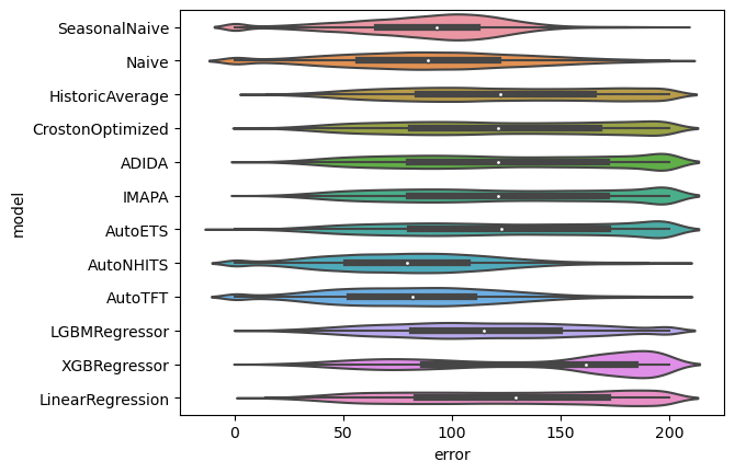
误差分布
!pip install seaborn
import matplotlib.pyplot as plt
import seaborn as sns
evaluation_df_melted = pd.melt(evaluation_df, id_vars=['unique_id', 'cutoff', 'metric'], var_name='model', value_name='error')
SMAPE
sns.violinplot(evaluation_df_melted.query('metric=="smape"'), x='error', y='model')
为时序组合选择模型
特征:
- 一个统一的 dataframe,包含了所有不同模型的预测
- 容易组装
- 平均预测
- 或者MinMax(选择是集成)
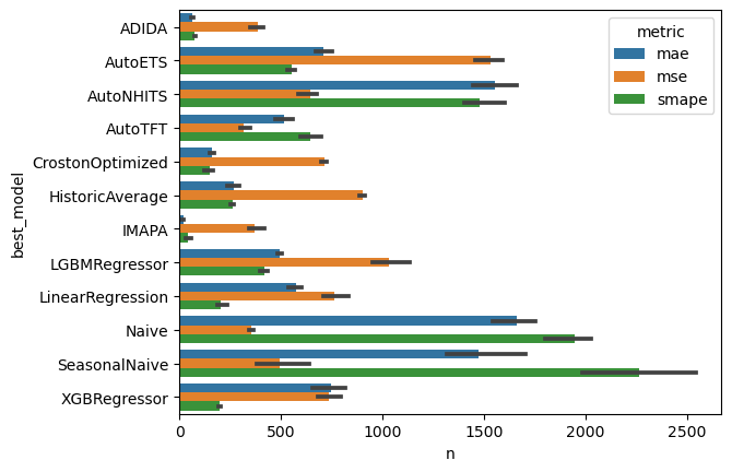
# Choose the best model for each time series, metric, and cross validation window
evaluation_df['best_model'] = evaluation_df.idxmin(axis=1, numeric_only=True)
# count how many times a model wins per metric and cross validation window
count_best_model = evaluation_df.groupby(['cutoff', 'metric', 'best_model']).size().rename('n').to_frame().reset_index()
# plot results
sns.barplot(count_best_model, x='n', y='best_model', hue='metric')
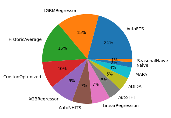
多元一体1:一个包容性的预测饼图
# For the mse, calculate how many times a model wins
eval_series_df = evaluation_df.query('metric == "mse"').groupby(['unique_id']).mean(numeric_only=True)
eval_series_df['best_model'] = eval_series_df.idxmin(axis=1)
counts_series = eval_series_df.value_counts('best_model')
plt.pie(counts_series, labels=counts_series.index, autopct='%.0f%%')
plt.show()
sf.plot(Y_df, cv_df.drop(columns=['cutoff', 'y']),
        max_insample_length=28 * 6,
        models=['AutoNHITS'],
        unique_ids=eval_series_df.query('best_model == "AutoNHITS"').index[:8])
为不同时序分组选择不同的预测方法
# Merge the best model per time series dataframe
# and filter the forecasts based on that dataframe
# for each time series
fcst_df = pd.melt(fcst_df.set_index('unique_id'), id_vars=['ds'], var_name='model', value_name='forecast', ignore_index=False)
fcst_df = fcst_df.join(eval_series_df[['best_model']])
fcst_df[['model', 'pred-interval']] = fcst_df['model'].str.split('-', expand=True, n=1)
fcst_df = fcst_df.query('model == best_model')
fcst_df['name'] = [f'forecast-{x}' if x is not None else 'forecast' for x in fcst_df['pred-interval']]
fcst_df = pd.pivot_table(fcst_df, index=['unique_id', 'ds'], values=['forecast'], columns=['name']).droplevel(0, axis=1).reset_index()
sf.plot(Y_df, fcst_df, max_insample_length=28 * 3)
-
"Et pluribus unum" 是拉丁语,意思是"合众为一"或"多中之一"。这句话是美国的传统格言,出现在美国国徽上,也曾经是美国的非正式国家座右铭(直到1956年被"In God We Trust"取代)。它表达的理念是:许多不同的州或人民团结成为一个统一的国家。 ↩